Getting Started#
Installation#
To use magtomo, first install it using pip:
(.venv) $ pip install magtomo
Examples#
The examples included here are lightweight demonstrations, making use of a small array (32, 64, 32) and 72 projections to produce vector and orientation reconstructions (18 projections for scalar reconstruction).
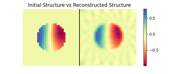
Scalar Tomography#
The magtomo.examples.scalar_tomo() function performs an example 3D scalar reconstruction. First, projections are
collected as the sample is rotated around the y axis according to the provided angles. Then, the projections are used
to call the inversion function, recovering the initial structure
# calculated projections for the 3D structure
# at the desired angles creates projections
projections = radon(struct, angles)
# uses the projections (and angles at which
# the projections were taken) to recover the initial structure
recons = inv_radon(projections, angles)
A comparison of the initial and reconstructed structures is shown below (obtained with 18 total projections). More projections can be used for improved reconstruction quality.
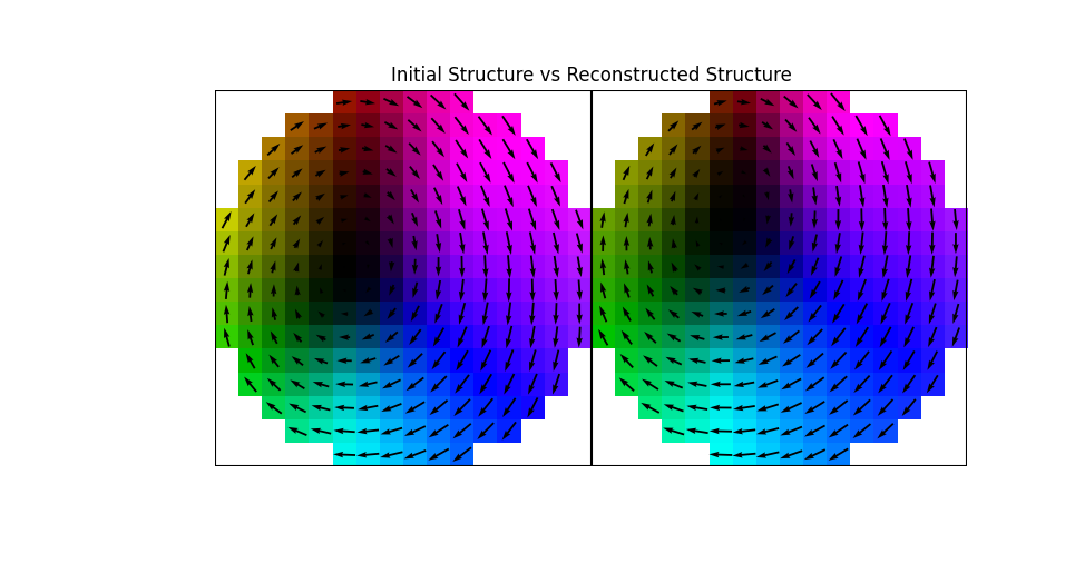
Vector Tomography (XMCD)#
In vector tomography (in this case x-ray magnetic circular dichroic tomography), using circularly polarized light gives
access to the component of the magnetization parallel or anti-parallel to the beam. To simulate projections from a
structure, an magtomo.Experiment.Experiment class is created.
The polarization, an argument for the class constructor, determines the type of interaction. Circularly polarized light
is indicated with complex 1j (circular left) and -1j (circular right). The exam
The magtomo.examples.vector_tomo() function performs an example 3D vector or orientation tomographic
reconstruction. The process is similar to Scalar Tomography; appropriate projections are calculated and then used
as input for the reconstruction. For simulating dichroic tomography experiments, projections are calculated using the
magtomo.Experiment.Experiment class and reconstructed with the magtomo.Reconstruction.Reconstruction
class.
# create experiment class, defining the rotations and polarizations
exp = Experiment(magnetization=struct, rotations=rot, pol=pol)
exp.calculate_sinogram()    # calculate the projections
projections = exp.sinogram  # get the projections to be used an input

# create a reconstruction class
recons = Reconstruction(initial_guess, rotations=rot, projections=projections,
                        pol=pol, mask=mask)
recons.reconstruct()        # reconstruct (iterative gradient descent)
A comparison of the initial and reconstructed structure is shown below (obtained with 72 total projections). More projections and tilts can be used for improving the reconstruction quality.
Orientation Tomography (XMLD)#
In orientation tomography linearly polarized light is used to gain information about the orientation of charge and
magnetic anisotropies. Linearly polarized light can take integer values corresponding to the angle between the x axis
and the polarization. As before, Projections are simulated using the magtomo.Experiment.Experiment class and
subsequently reconstructed using the magtomo.Reconstruction.Reconstruction class.
In this example, two polarization are used, \(\pm45^\circ\) and two tilt axes, \(\pm30^\circ\). The same process
as the one outlined in Vector Tomography (XMCD) is followed with a different dichroism option when calling the
magtomo.examples.vector_tomo() function.
dichroism = 'LD' # circular ('CD') or linear ('LD')
A comparison of the initial and reconstructed structures is shown below (obtained with 72 total projections). More projections and tilts can be used for improving the reconstruction quality.
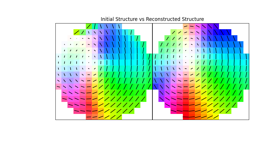
Orientation tomography generally requires more iterations for a successful reconstruction and is best performed with GPU acceleration. See code in Nature 636 354 for MATLAB version.
Full Code#
The full code from the examples.py file can be seen here:
View Code
import logging
import numpy as np
import magpack.rotations as rtn
import ThreeDViewer.data
from magtomo.Experiment import Experiment
from magtomo.Reconstruction import Reconstruction
from ThreeDViewer.image import plot_3d
from importlib import resources
from magtomo.radon import radon, inv_radon
from magpack import vectorop, structures, io


def vector_tomo(angles, tilts, kind='CD', it=10, learning=30):
    """ Examples of vector and orientation tomography.

    Parameters
    ----------
    angles : np.ndarray | list of float
        The tomographic rotation angles.
    tilts : np.ndarray | list of float
        The tomographic tilt angles.
    kind : {'CD', 'LD'}
        Vector (CD) or Orientation (LD) tomography options.
    it : int
        The number of gradient descent iterations to evaluate.
    learning : float
        The learning parameter for gradient descent.
    """

    # specify a structure
    struct = _get_structure()
    mask = vectorop.magnitude(struct) > 0

    # get rotation matrices
    rot = rtn.tomo_rot(angles, tilts)
    # get polarizations for each rotation
    pol_a = np.repeat(-45 if kind == 'LD' else 1j, rot.shape[0])
    pol_b = np.repeat(+45 if kind == 'LD' else -1j, rot.shape[0])

    # double rotations to match the polarizations
    pol = np.hstack((pol_a, pol_b))
    rot = np.concatenate((rot, rot), axis=0)
    # initialize the experiment class with the structure, rotation matrices and polarizations
    exp = Experiment(magnetization=struct, rotations=rot, pol=pol)
    # calculate and sinogram that will be used as input
    exp.calculate_sinogram()
    # plot the sinogram
    cmap = 'jet' if kind == 'LD' else 'Spectral'
    exp.plot_sinogram(cmap=cmap)
    # these projections will be used to attempt a reconstruction
    projections = exp.sinogram

    # provide an initial guess for the structure, LD is best with random initial conditions, CD with zero
    initial_guess = np.ones_like(struct) / np.sqrt(3)
    # initialize a reconstruction class and perform reconstruction
    recons = Reconstruction(initial_guess, rotations=rot, projections=projections, pol=pol, iterations=it,
                            mask=mask, learning_parameter=learning)
    recons.reconstruct()
    norm_recons = vectorop.normalize(recons.magnetization)

    sinogram_comparison = np.concatenate([recons.sinogram, exp.sinogram], axis=1)
    a = plot_3d(sinogram_comparison, show=False, cmap=cmap, axes_names=(r"$\theta$", "x", "y"), init_take=0)
    b = plot_3d(norm_recons, axial=True if kind == 'LD' else False, arrow_skip=1, show=False)
    c = plot_3d(struct, axial=True if kind == 'LD' else False, arrow_skip=1)


def scalar_tomo(angles):
    """Example of single axis scalar tomography."""
    # get a scalar field to reconstruct
    struct = _get_structure()[0]

    # calculate projections
    projections = radon(struct, angles)
    plot_3d(projections, cmap='Spectral', init_take=0, axes_names=(r"$\theta$", "x", "y"), title="Projections")

    # reconstruct the object from projections
    recons = inv_radon(projections, angles)

    a = plot_3d(struct, cmap='Spectral', init_take=1, init_slice=47, show=False, title="Initial Structure")
    b = plot_3d(recons, cmap='Spectral', init_take=1, init_slice=47, title="Reconstruction")


def _get_mask(shape):
    """Makes a cylinder mask for the provided (vector field) shape."""
    xx, yy, zz = structures.create_mesh(*shape[-3:])
    r = np.sqrt(xx ** 2 + zz ** 2) < shape[1] / 4  # radius mask based on the x size
    h = shape[2] // 4 > np.abs(yy)  # radius mask based on the y size
    return r * h


def _get_structure():
    """Returns an example magnetization vector field from the ThreeDViewer package."""
    data_path_resource = resources.files(ThreeDViewer.data) / 'cylinder.ovf'
    with data_path_resource as resource:
        data = io.load_ovf(resource).magnetization

    # make y out-of-plane to match the tomography coordinate system
    data = np.array(data[[1, 2, 0]].transpose((0, 2, 3, 1)))
    # mask to leave room for tilting
    return data * _get_mask(data.shape)


def _evenly_spaced(initial, final, steps):
    """Creates an evenly spaced array assuming the ends are cyclic."""
    dx = (final - initial) / steps
    return np.linspace(initial, final - dx, steps)


if __name__ == '__main__':
    logging.basicConfig(level=logging.INFO)
    initial_angle, final_angle, angle_steps = 0, 360, 18
    rotation_angles = _evenly_spaced(initial_angle, final_angle, angle_steps)

    # example of scalar tomography
    scalar_tomo(rotation_angles)

    # example of vector or orientation tomography
    tilt_angles = [30, -30]
    iteration_number = 10
    learn_param = 30
    dichroism = 'CD'  # circular ('CD') or linear ('LD')
    vector_tomo(rotation_angles, tilt_angles, kind=dichroism, it=iteration_number, learning=learn_param)